|
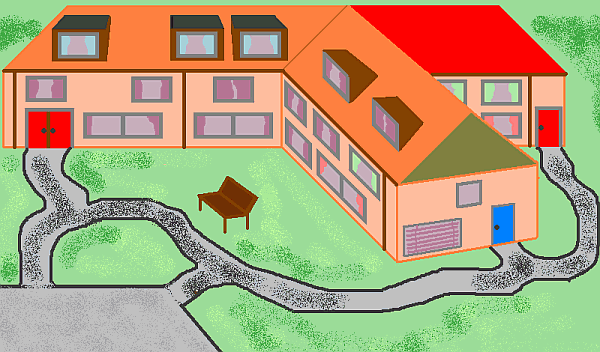
Specialist Dementia Residential Home |

|
| Capacity 75 residents. |
| Lesson Aim: | What Chi Squared testing can suggest and what it cannot and its background |
| Lesson Objective: | Students will (along with the presentation) respond to calculations of Chi Squared method and wider talked through implications of bell curves (statistics and the insurance industry etc. and chaotic systems that cannot be insured as there is no bell curve). |
| Time: | 20 minutes |
| There are qualitative and quantitative research methods. Qualitative methods produce in depth statements that are tested for validity; quantitative methods produce broad returns of figures that are tested for reliability - repetition of returns and stability of returns of data perhaps over long periods or many examples. |
| Reliable data delivers distributions that become expected. What happens when observed data suddenly deviates unexpectedly from previous and well established data that forms expectations? |
|
Specialist Dementia Residential Home |
|
| Capacity 75 residents. |
|
This last year January had an unexpected rise in deaths. Was this statistically significant and if so what does this mean?
The fact is that residents are nearing and at the end of their lives with rapidly declining faculties and many are expected to die each month. Who dies depends on their individual conditions. Some die soon after admittance. A few die after several years. Most live just months. The actual number dying can be worked out from the bell curve below. We notice over the years that this distributes out so that in the month of January one in ten do die. We have an expectation evidenced over time that 10% of residents die in that month. There are 75 people in the home, at capacity, and, because of increasing demand, every time someone dies someone new comes into the home the very next day. Last January 16 people died (21.3333%). Yet we know that normally the figure does keep remarkably to 10% and that this is the normal distribution figure in the home in January year on year. What is 10% of 75? This means that some years 8 die and some years 7 die, but if 6 die one year then it happens 9 will die another. Yet this year we have 16! |
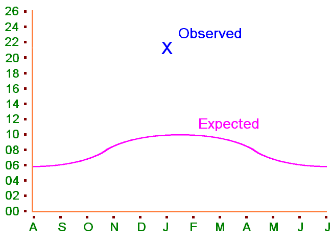
| Statistically speaking, is this likely to happen by chance? We need a firmer question: by what probability could this happen simply by chance? |
| If it is improbable by chance we might have to open an investigation about what happened and potentially what is going wrong in the home. |
| Question One. | How many people out of 75 would you expect to die? |
| Question Two. | How many people out of 75 would you expect to live? |
| Question Three. | How many people out of the 75 did die? |
| Question Four. | How many people out of the 75 did live? |
|
We need to make a table of this: Categories - Alive, then Dead Observed (for Alive, for Dead) Expected (for Alive, for Dead). |
| Category | Observed |
Expected (10% should die) |
| Alive | 59 | 67.5 |
| Dead | 16 | 7.5 |
| Total | 75 | 75 |
| 1. |
For each category compute the difference between observed and expected counts.
(O-E) |
| 2. |
For each category, square that difference - same as multiply by itself.
(O-E)2 or (O-E) * (O-E) |
| 3. |
Divide by the expected count in each case.
(O-E)2/E |
| 4. |
Add the values for all categories. In other words, compute the sum of each.
Category 1 (O-E)2/E + Category 2 (O-E)2/E |
| 5. |
Use a table (or computer program/ webpage) to calculate the P value based on the number of degrees of freedom (which is the number of categories minus 1).
Degrees of freedom = categories - 1 |
| For our Residential Home the categories are Alive and Dead. |
|
Dead: (Observed-Expected) Squared divided by Expected (O-E)2/E 16 Observed Dead minus 7.5 Expected Dead equals 8.5 (16 - 7.5) = 8.5 8.5 multiplied by 8.5 equals 72.25 8.5 * 8.5 = 72.25 72.25 divided by 7.5 Expected Dead equals 9.633 72.25 / 7.5 = 9.6333 In short: (16 - 7.5) * (16 - 7.5) / 7.5 = 9.6333 |
| Hold that figure! 9.6333 |
|
Alive: (Observed-Expected) Squared divided by Expected
59 Observed Alive minus 67.5 Expected Alive equals -8.5 (59 - 67.5) = -8.5 -8.5 multiplied by -8.5 equals 72.25 [positive!] -8.5 * -8.5 = 72.25 72.25 divided by 67.5 Expected Alive equals 1.0703 72.25 / 67.5 = 1.0703 In short: (59 - 67.5) * (59 - 67.5) / 67.5 = 1.0703 |
| Hold that figure! 1.0703 |
|
Alive result plus Dead result = X2 VALUE 9.6333 plus 1.0703 equals 10.7036 9.6333 + 1.0703 = 10.7036 |
| X2 VALUE is 10.7036 |
| Number of degrees of freedom = number of categories minus 1 |
| Null hypothesis is where the outcome equals with what you would expect within the degrees of freedom. |
|
Go to Chi squared table on n-1, and thus with just two categories we have 1 degree of freedom. So that is top of the table (1) and there are probability measures. 10.7036 is just under 0.001 or 1 in 1000.
In fact QuickCalcs calculates this to 10.704 and a P value of 0.0011 which is very statistically significant. It is 1 in 1100. |
| This seems very unlikely! |
| Given that this outcome is so slight as chance (yet it could still BE chance) what should one do about the specialist old people's home? |
| Such a statistical outcome only SUGGESTS an additional reason for such variation from expectation, but the qualitative answer behind such a quirk needs investigating. |
| Strictly speaking two categories (n-1 = 1) should not be used, but there is a Yates correction for such one degree of freedom. It is to subtract 0.5 from each calculated value of O-E regardless of plus or minus before proceeding further. |
|
((16 - 7.5) - 0.5)*((16 - 7.5) -0.5) / 7.5 = 8.5333 or 8 * 8 / 7.5 = 8.5333 ((59 - 67.5) - 0.5)*((59 - 67.5) - 0.5) / 67.5 = 1.2 or -9 * -9 / 67.5 = 1.2 8.5333 + 1.2 = 9.7333 with Yates correction [was 10.7036] |
| The correction increases the chance that such a variation can happen without additional incident - it increases the allowed variation. |
| You will see references to chi squared (sometimes chi square or chi-square) often in analysis of statistics. How do you respond to this? Read it over again and try your own simple example. |